One-Dimensional Kinematics

Between the idea and the reality, between the motion and the act, falls the shadow.

— T.S. Eliot, The Hollow Men

The term kinematic is the English version of the French word cinématique, which is derived from the Greek κίνημα, or kinema, meaning motion, itself being derived from κινεῖν, or kinein, which means to move.

In this tutorial we will learn about one-dimensional kinematics, i.e., the motion on a straight line, of point particles. In the following, each time an object is mentioned, the object is thought of as a single point particle.

Distance and Displacement

To define movement, a coordinate system must be set up first. In all the basic tutorials, the entire action takes place in the standard Euclidean plane or the standard Euclidean space , each time equipped with the standard Euclidean scalar product.

When objects move, they cover a certain distance, which is defined as the total length of travel, and measured in metres (m). The displacement is defined as the change in position of an object over time, and also measured in metres. Let and , with , be two fixed moments in time and and be the positions of an object at those exact times, then the displacement of the object is defined as: Please note that while the distance covered is always positive, the displacement might be zero or even negative.

Imagine going to the computer store, which is, luckily, only away, on a straight line, to buy a new GPU and immediately returning home afterwards, once again, on a straight line, then the total displacement is , as , but the distance covered obviously is equal to . A negative displacement simply means movement in the negative direction, as defined by the coordinate system.

Defining the position of an object to be a mathematical function of time, , , mapping an instant of time to the actual position of the object at that exact time, the motion of an object can be visualized by the graph of the function.

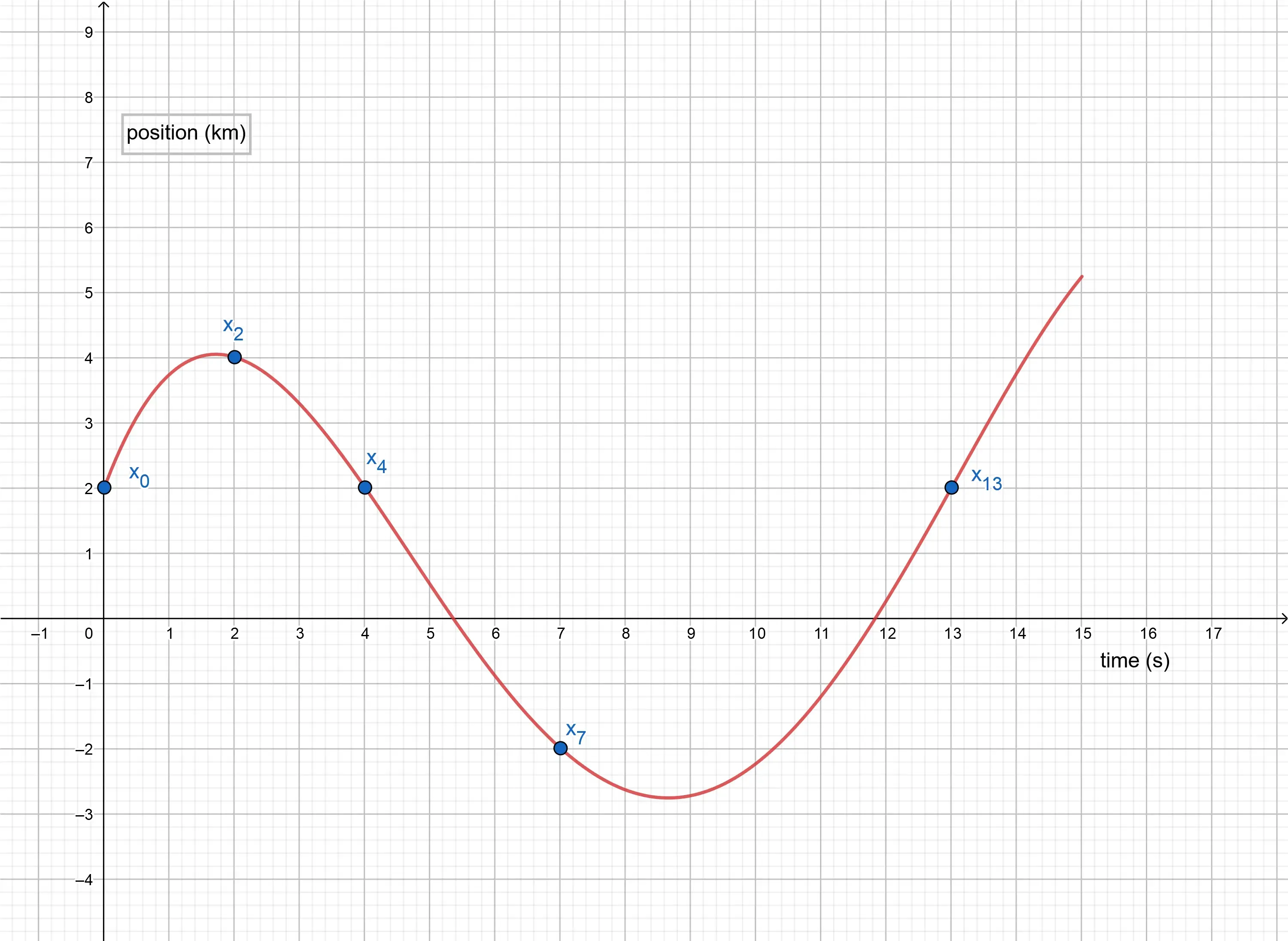
In the above graph one can see that while between and the object travels 4 km, its total displacement is , indicating that it moved an equal distance in the positive and negative direction. Between and , the total distance travelled by the object is , the displacement is negative, however, indicating a movement in the negative direction (to the left in the first figure of this tutorial): . Between and , the distance travelled is once again , and the displacement is positive , indicating a movement in the positive direction (to the right).

Average Speed and Velocity

Often it is not enough to know how far an object has travelled, but the time it took for the object to reach its destination is important as well. This is called the average speed of an object. Let be the distance covered and be the elapsed time, then the average speed is defined as , and measured in, obviously, meters per second (). Note that since both the distance and the elapsed time are always positive, so is the average speed.

Yet, even knowing the average speed of an object is frequently not satisfying enough. It is also essential to know how fast an object was moving between certain points in time. This measure is called the average velocity of an object and is defined as the displacement per time. Let be the position of an object at the time and its position at the time (some time after , i.e. ), then its average velocity is defined as . Note that, unlike the average speed, the average velocity also indicates the direction the object is travelling in, as the average velocity is actually negative, if and only if, , as depicted in the figure below.

‌

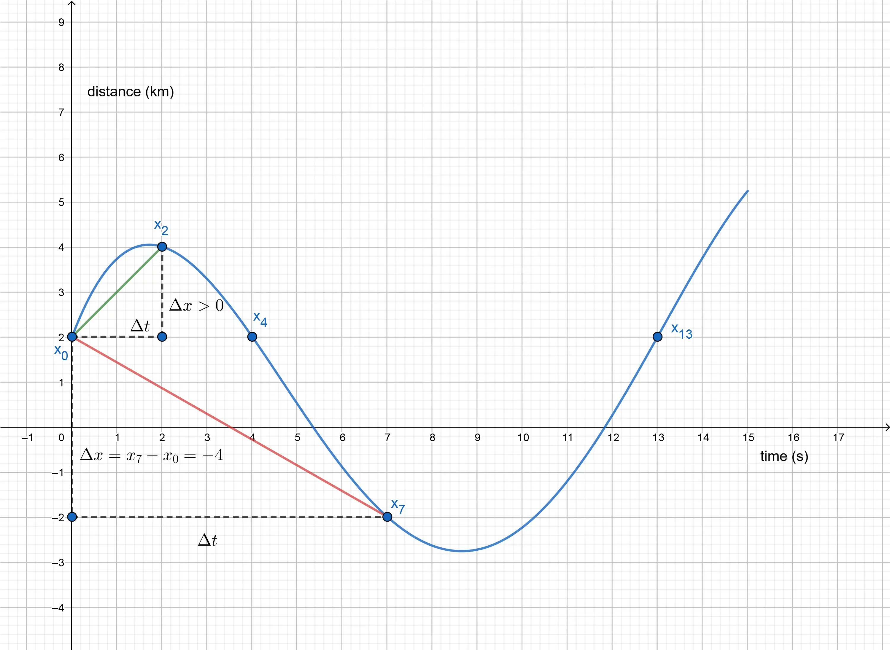
In the figure, one can also see that the slope of a line connecting two points is equal to the average velocity during that time interval.

Considering the velocity to be a mathematical function of time, , , mapping an instant of time to the velocity of an object at that time, the average velocity can be defined in a more precise way as a definite integral. Let and be two instants of time, then the average velocity between those time intervals is

Instantaneous Velocity

Even the average velocity of an object does not hold enough information, as most often objects do not travel at the same velocity all the time (just imagine driving a car) — their velocity changes constantly. It is ideally desirable to know the velocity of an object at each instant of time (not only during certain time intervals). This is called the * instantaneous velocity*, , and can be defined by considering smaller and smaller time intervals, or mathematically: Note that the magnitude of the instantaneous velocity is called the instantaneous speed (think of the speedometer in a car). The instantaneous velocity can also be interpreted as the velocity that an object would continue to travel at, if no forces, no longer interacted with it.

Geometrically, the instant velocity at the time is the slope of the tangent line at :

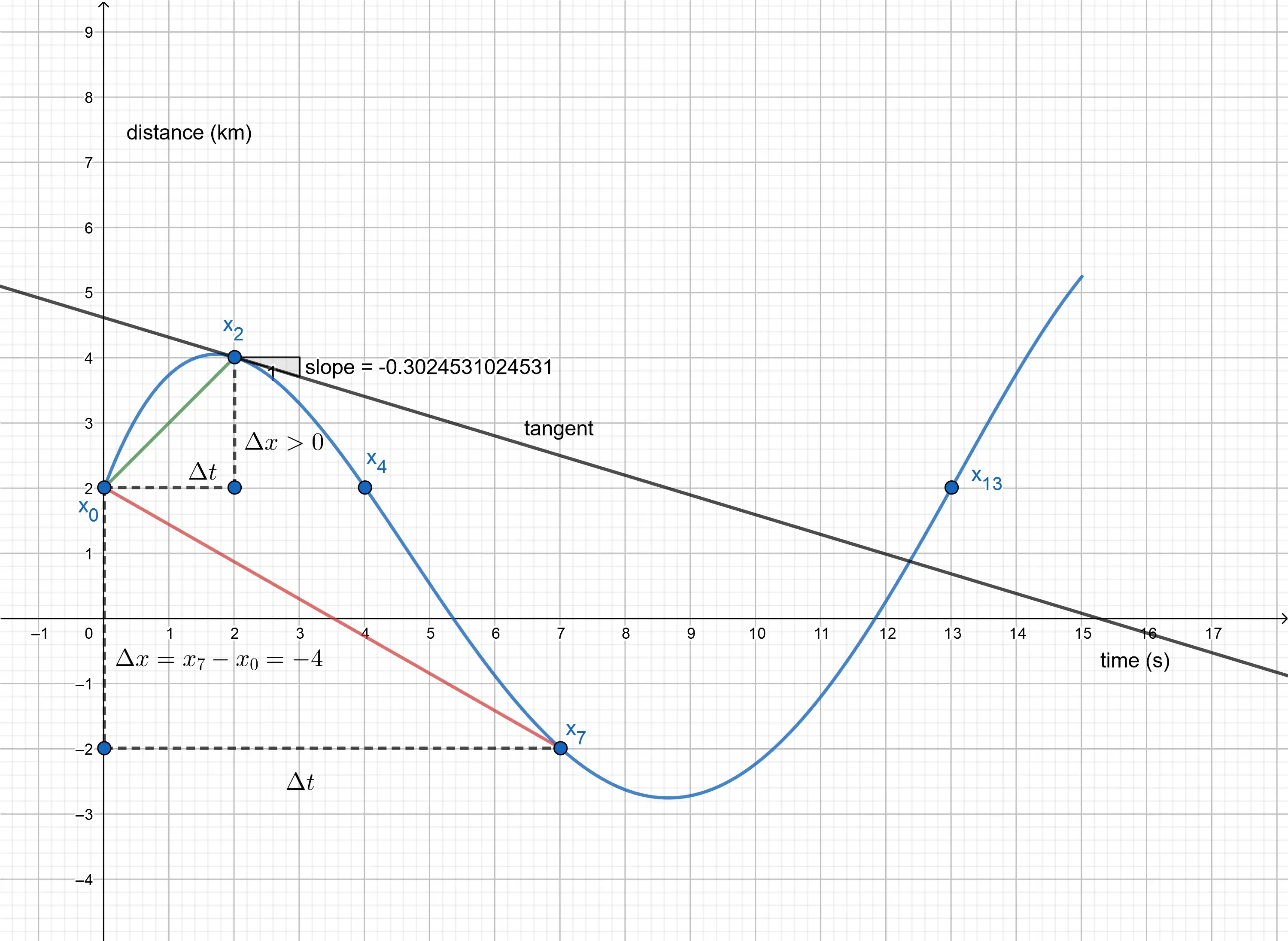
To be more precise, the instantaneous velocity of an object, at any particular moment in time, can be expressed as the derivative of the position with respect to time:

Drawing the graph of the velocity function, one can see that the displacement of an object can be expressed as the area under the graph between two time points, or, the displacement function is the integral of the velocity function :

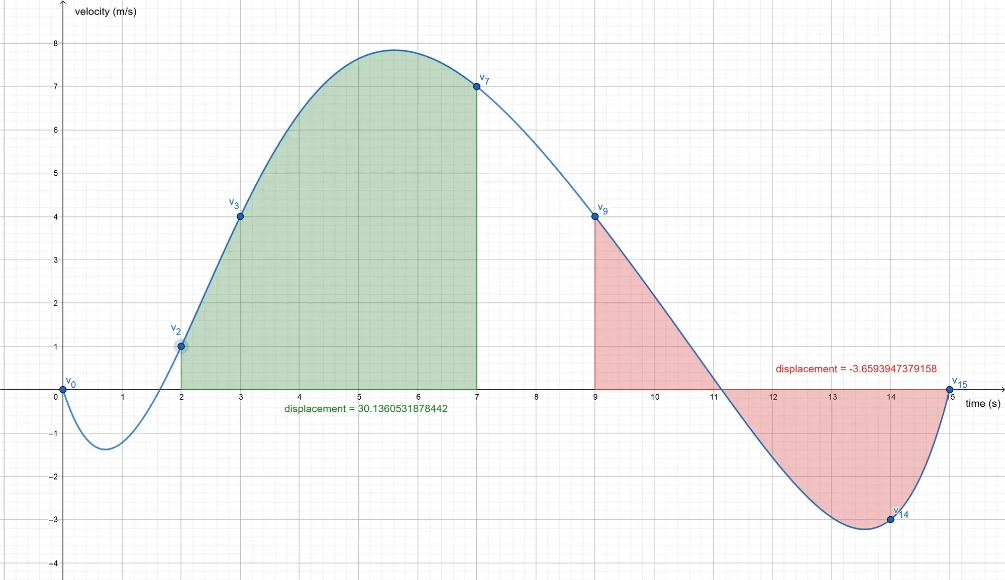
A negative velocity simply means that the object is speeding ahead in the negative direction, as defined by the underlying vector space.

Between and , the area under the graph of the function is positive, meaning the object mostly in the positive direction, whereas the area between the graph and the -axis is negative between and , indicating a net movement in the negative direction.

Acceleration

As velocity describes the change of position over time, acceleration is the rate of change of velocity over time. The concept of acceleration is one of the most important concepts in classical physics. In later chapters we will learn that Galileo showed that falling bodies move with constant acceleration and how Newton managed to find a relation between acceleration and force. It is thus essential to have a good understanding of the concept of acceleration.

The average acceleration is defined analogously to the average velocity. Let and be the velocities of an object measured at times , then the average acceleration, , is defined as The acceleration of an object is thus measured in meters per second squared: .

Similarly to the instantaneous velocity, the instantaneous acceleration, , at a specific time, can be computed by taking smaller and smaller time intervals: .

Note that, in one dimension, if the velocity and the acceleration of an object have the same sign, the speed of the object increases. When the velocity and the acceleration have opposite signs, the speed of the object decreases.

To be mathematically more precise, the instantaneous acceleration at a point in time is defined as the derivative of velocity with respect to time: . The velocity can then be considered as the area under the graph of the acceleration function , , mapping an instant of time to the acceleration of an object at that exact time, or, thinking about integrals again, the velocity is the integral of the acceleration with respect to the time: .

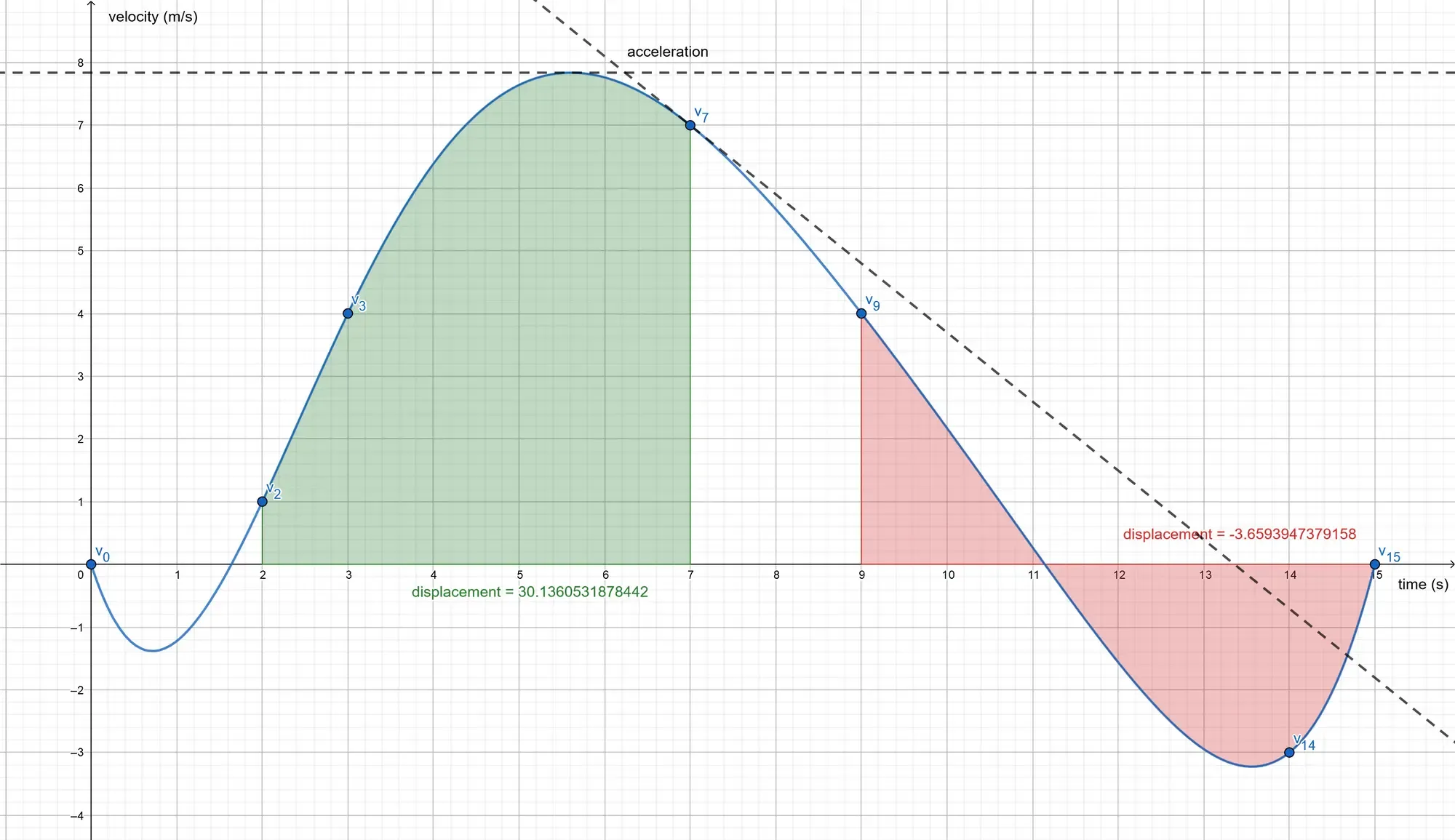
The figure above shows the acceleration as the slope of the tangent at a specific point. One can see that at the peak of its velocity, the object has no acceleration for a brief moment of time (tangent line parallel to the -axis), and the negative slope means a negative acceleration, which corresponds to the object losing velocity, i.e. slowing down.

Motion with Uniform Acceleration

In the case of uniform or constant acceleration, it is relatively easy to derive simple formulas to describe the motion of an object. In an idealized world, without friction, for example, motion with constant acceleration can be used to model a wide range of everyday phenomena.

If an object has constant acceleration, its average and instantaneous accelerations are obviously the same. Let be two arbitrary chosen times, then . Since the choice of time is not significant for constant acceleration, it seems wise to set , simplifying the formula to where is the initial velocity of the object. It is thus possible to express the velocity of an object as an affine function of time: , which means that the velocity of an object at time is the initial velocity plus times its acceleration.

The next question to ask is how far an object moves in a given time. Using the same simplification as above, the formula of the average velocity reduces to , thus . Since in the case of constant acceleration, the average velocity is simply the average of the initial and final velocities, this formula can be further simplified to express the position of an object as an affine function of time: .

Finally, substituting , the formula to compute the position of an object after a certain time , under constant acceleration, looks as follows: .

Implementing motion with uniform acceleration in C++ is now straightforward:

float Kinematics::posUM(const float x0, const float v0, const float a, float dt)
{
  return x0 + v0 * dt + 0.5f * a * dt * dt;
}

Free Fall

Free fall, the motion of an object falling freely under the influence of gravity and gravity alone, is probably the most famous example of motion with constant gravity. Galileo was most likely the first to postulate that falling bodies moved with constant acceleration. The acceleration produced by the gravity, , on Earth is about , thus, if is set to (by moving the centre of the coordinate system, if you are so inclined), the formula to compute the position of an object in free fall after a certain time is as easy as .

Hamiltonian Systems and Symplectic Integration

As stated above, the problem of an object in motion is a classical mechanical problem. Recall that and were defined as two functions determining the position and velocity of an object at any time . Let further and be the derivative and the second derivative of the position function. Newton declared that all motions of a system are uniquely determined by their initials positions and initial velocities, given by the derivative of the position (). In particular, the initial position and velocity uniquely determine the acceleration, in other words, there is a function such, that . This equation is called Newton’s equation of motion. For a mathematically more precise introduction into the equation of motion, refer to the tutorial Galileo versus Newton ([[galileoNewton]] Galileo vs. Newton).

By the year 1833, Sir William Hamilton had invented a new theory to reformulate those classical mechanical problems in a more modern way, providing a more abstract understanding of the theory. The main advantage of this new theory comes from the symplectic structure of Hamiltonian systems.

Newton’s equation of motion takes the form: which can be transformed into a system of differential equations of the first order which can then be written as where and are given functions (the velocity and acceleration functions, which can both vary over time). Those two functions are symplectomorphisms, which means that they conserve the symplectic two-form .

The equations of motion take this form if the Hamiltonian is of the form , where is the sum of all kinetic and the sum of all potential energy, which happens to be the case in this situation.

The goal of this tutorial is not to give an introduction into Hamiltonian Systems, but rather to solve the equations of motion, thus, given the initial conditions (the initial position of the object) and (the initial velocity of the object), how can the above so-called system of differential equations be solved algorithmically, i.e. how do we compute the position and velocity of our game objects at any given moment in time?

Numerical Integration and Implementation

To algorithmically, or numerically, solve the above system of differential equations, the equations of motion, a technique called numerical integration is used. Numerical integration basically repeats certain small steps again and again, i.e., in this case, objects start at an initial position with an initial velocity and then, using small-time steps, the new velocity and position are computed, which are then set as the new initial positions and velocities. Thus, numerical integration tries to find an approximate discrete solution to a continuous problem by iteration.

One such approximate discrete solution of the Hamiltonian equations of motion can be produced by iterating and where is the time step and denotes the time after steps.

This technique is called semi-implicit Euler integration, named after the Swiss mathematician Leonhard Euler. This integration technique is a symplectic integrator, which means it is well suited to solve Hamiltonian systems, i.e. it also conserves the symplectic form , which means that it can conserve the energy of the system quite well.

Note that to compute the position of the object at the time , the velocity at the time is used instead of the velocity at the time . Using the velocity at the time instead, leads to the standard Euler method, which is not a symplectic integrator, though. As a consequence, the symplectic semi-implicit Euler method almost conserves the energy of the Hamiltonian system, while, very often, the energy increases steadily when using the standard Euler method, resulting in a loss of accuracy.

After all that scary talk about abstract mathematics, implementing the semi-implicit Euler method to solve the equations of motions is actually straightforward:

void Kinematics::semiImplicitEuler(float& pos, float& vel, const float acc, const float dt)
{
  vel += acc * dt;
  pos += vel * dt;
}

As an example, assume that nine bullets are shot from guns positioned at the left of the screen. The initial positions of the centres of the bullets are stored in an array called centres, the initial velocities are stored in the velocities array and the accelerations in the accelerations array. The motion of the bullets can then be modelled as follows, just please note that in a game, the position, and velocity are obviously measured in pixels, or pixels per second, instead of meters and meters per second: 1 pixel usually corresponds to about :

const float Kinematics::metersPerPixel = 0.000264583f;    // 1 pixel = 0.000264583 meters

util::Expected<void> PlayState::update(const double deltaTime)
{
  if (isPaused)
    return { };

  // get meters per pixel
  const float mpp = physics::Kinematics::metersPerPixel;

  // update position based on symplectic integration of the equations of motion
  for (unsigned int i = 0; i < centers.size(); i++)
  {
    // the "even" bullets move with non-constant acceleration
    if (i % 2 != 0)
      accelerations[i] += rand()%10 * mpp;

    // symplectic integrator: semi-implicit Euler
    physics::Kinematics::semiImplicitEuler(centers[i].x, velocities[i], accelerations[i], deltaTime);

    // wrap screen
    if (centres[i].x > dxApp.getGraphicsComponent().getCurrentWidth())
    {
      centres[i].x = 0.0f;
      accelerations[i] = rand()%10 * mpp;
      velocities[i] = rand()%100 * mpp;
    }
  }

  // return success
  return { };
}

util::Expected<void> PlayState::render(const double farSeer)
{
  // let the far seer update the positions if necessary
  for (unsigned int i = 0; i < centers.size(); i++)
    centers[i].x += velocities[i]*farSeer;

  // render circles
  for (unsigned int i = 0; i < centers.size(); i++)
    dxApp.getGraphicsComponent().get2DComponent().drawEllipse(centers[i].x, centers[i].y, 10.0f, 2.5f);

  // print FPS information
  dxApp.getGraphicsComponent().getWriteComponent().printFPS();

  // return success
  return { };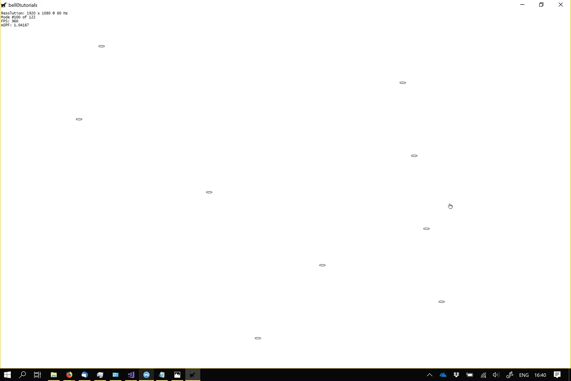
}

That’s it. All in all, one-dimensional kinematics are rather easy to handle, but the theory behind Hamiltonian systems and symplectic integrators can be a bit intimidating. Just remember to update the velocity before updating the position, and you are all set!

References

• Dynamical Systems, Prof. Dr. K.-F. Siburg
• Dynamical Systems, C. Robinson
• Geogebra
• Physics, by James S. Walker
• Tricks of the Windows Programming Gurus, by A. LaMothe
• Wikipedia