The Berlekamp-Massey Algorithm

This tutorial introduces linear feedback shift registers (LFSR) and explains the Berlekamp - Massey algorithm to find the shortest LFSR for a given binary output sequence. An implementation of the algorithm in C++ is provided as well.

Feedback Shift Registers

Feedback shift registers, or FSRs, for short, were probably first invented by Solomon Golomb and Robert Tausworthe. This tutorial is but a brief introduction to the theory of FSRs. We will learn, however, how to find the shortest linear FSR for a given binary output sequence.

An FSR of length is specified by a Boolean function , the so-called feedback function. Let …, be the initial input stream for such a shift register, then the output consists of the rightmost bit , while all the other bits are shifted to the right by one position. The leftmost cell is then filled by the new bit …, . Thus the shift register can be fully defined by the recursive formula for .

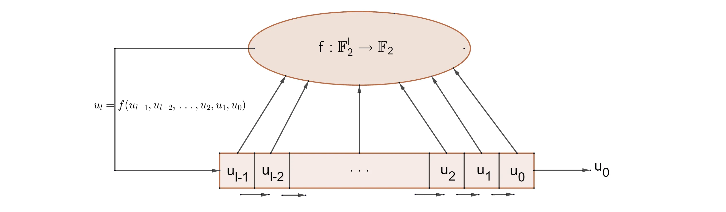
The first bits , , …, are called the start value, or the seed, of the FSR and the key expansion transforms the short sequence of length , which is called the effective key, into a key stream of arbitrary length. In a cryptographic context, those bits form the secret key system.

The simplest and best understood FSRs are the so-called linear-feedback shift register, or LFSRs. The feedback function of LSFRs is a linear map.

Linear Maps

A boolean function is called a linear form, if its degree is and its absolutely term is , and is thus of the form , where for all . Over a linear form is thus a partial sum where .

It is easy to see that there are exactly Boolean linear forms in variables and they naturally correspond to the power set .

Boolean linear functions are actual linear mappings in the sense of linear algebra, that is, a boolean linear function is a linear map, if and only if, for all and : and .

Using a linear map, the iteration of the shift registers takes the following form: . Obviously, the operation of such a register is deterministic, and thus the seed completely defines how the register works. Likewise, because the register has but a finite number of possible states, it must eventually enter a repeating cycle. Nonetheless, with a well-chosen feedback function, LFSRs can produce long cycles of bits that appear to be pseudo-random.

Fibonacci LFSRs

The Fibonacci LFSR only feeds a few bits back into the feedback function. Those bits that actually affect the next state are called taps. The taps are then XORed, which is equivalent to the addition in , with the output bit and then fed back into the leftmost bit. The information about the taps can be represented using a polynomial in , the so-called feedback polynomial . For example, in a 16-bit LFSR, the following polynomial defines the st, rd, th and th bits as the taps: .

The LFSR is said to be of maximal length, if, and only if, the corresponding feedback polynomial is primitive. The above polynomial is indeed primitive.

The following C++-code creates a -bit LFSR with a given feedback polynomial:

// 16-bit Fibonacci Linear-Feedback Shift Register defined by a feedback polynomial
unsigned int lfsrFib16(uint16_t& seed, std::vector<int> feedbackPolynomial, std::string& output, int steps)
{
  uint16_t lfsr = seed;      // the initial seed for the LFSR defined by the feedbackPolynomial
  uint16_t bit = 0;        // the output of the linear feedback function
  unsigned int cycle = 0;      // the cycle length of the LSFR
  unsigned int size = feedbackPolynomial.size();
  do
  {
    bit = 0;
    // compute the new (leftmost) bit using the tabs defined by the primitive feedback polynomial
    for (unsigned int i = 1; i < size; i++)
      if (feedbackPolynomial[i] != 0)
        bit ^= (lfsr >> (size - 1 - i));

    // output the rightmost bit, and set the last bit to the newly computed bit
    output.push_back(std::to_string(lfsr%2)[0]);
    lfsr = (lfsr >> 1) | (bit << 15);

    // increase the period
    cycle++;
    steps--;
  } while (lfsr != seed && (steps > 0 || steps < 0));
  seed = lfsr;
  output.swap(output);
  return cycle;
}

The code is rather self-explanatory. The first actual line of code, inside the „do-while“ loop, simply takes the bits that are tapped, as defined by the feedback polynomial, and computes their sum by XORing them. The second line then „outputs“ the rightmost bit, by shifting everything to the right, and then replaces the last bit of the LSFR by the output of the feedback function just calculated in the first step. Note that by invoking the LSFR with a negative number for „steps“, the LFSR will continue to output bits until it has reached the end of its cycle, whose length it will return.

As an example, let us create a LFSR with the polynomial from above:

int main()
{
  // define the feedback polynomial: X^16 + X^12 + X^3 + X + 1
  std::vector<int> feedbackPolynomial;
  for (unsigned int i = 0; i < 17; i++)
    feedbackPolynomial.push_back(0);
  feedbackPolynomial[0] = 1;
  feedbackPolynomial[1] = 1;
  feedbackPolynomial[3] = 1;
  feedbackPolynomial[12] = 1;
  feedbackPolynomial[16] = 1;

  // set the seed (initial state of the LFSR)
  uint16_t seed = 0xB9B9;              // the initial seed

  // create the output vector
  std::string output;

  // print starting message
  std::cout << "Creating a LFSR with ";
  outputFeedbackPolynomial(feedbackPolynomial);
  std::cout << "Seed: " << std::bitset<16>(seed) << std::endl << std::endl;

  // let the feedback shift register work
  unsigned int steps = 25;
  lfsrFib16(seed, feedbackPolynomial, output, steps);
  std::cout << "Output after " << steps << " steps: ";
  std::cout << output << std::endl;

  return 0;
}

And here is the output:

Creating a LFSR with Feedback Polynomial:  X^16 + X^12 + X^3 + X + 1
Seed: 1011100110111001

Output after 25 steps: 1001110110011101010010011

Matrix Form

Binary LFSRs can be expressed by matrices in , by using the Frobenius companion matrix of the monic feedback polynomial. Let be a monic feedback polynomial, then the companion matrix is defined as

Let further be the seed of the LFSR, then the state of the LFSR after k steps is given by:

thus the Frobenius matrix completely determines the behaviour of the LFSR. Using matrix notation, it is straightforward to generalize LFSR to arbitrary fields.

Applications and Weakness

LFSRs can be implemented in hardware, which makes them very useful for on-the-field deployment, as they generate pseudo-random sequences very quickly, and this makes them useful in applications that require very fast generation of a pseudo-random sequence, such as direct-sequence spread spectrum (DSSS) radios, for example. One example of a DSSS is the IEEE 802. 11b specification used in wireless networks.

LFSRs have also been used for generating an approximation of white noise in various programmable sound generators.

LFSRs have long been used as pseudo-random number generators for use in stream ciphers, especially in the military, due to the ease of construction from simple electromechanical or electronic circuits. Unfortunately, with their linearity comes a huge weakness. Even just a small piece of the output stream is enough to reconstruct an identical LSFR using the Berlekamp - Massey algorithm. Obviously, once the LFSR is known, the entire output stream is known.

Important LFSR-based stream ciphers still in use nowadays include the A5/1 and the A5/2 ciphers used in GSM cell phones, or the E0 cipher used in Bluetooth. The A5/2 cipher has been broken and both A5/1 and E0 have serious weaknesses.

The Berlekamp - Massey Algorithm

Now that we know how to construct a LSFR, let us learn how to reconstruct one from knowing an output bit string. The first idea that comes to mind, obviously, is to abuse the linearity of the LFSR. Assume, further, that the length of the LSFR is known, then it is clear that a simple matrix inversion is enough to reconstruct the feedback polynomial. The difficulty then is to find the length of the LFSR.

Enter the Berlekamp — Massey algorithm. Basically speaking, this algorithm starts with the assumption that the length of the LSFR is , and then iteratively tries to generate the known sequence and if it succeeds, everything is well, if not, must be increased. The following explanations follow the original paper of Berlekamp.

To solve a set of linear equations of the form a potential instance of is constructed step by step. Let denote such a potential candidate, it is sometimes also called the „connection polynomial“ or the „error locator polynomial“ for errors, and defined as The goal of the Berlekemp — Massey algorithm is to now determine the minimal degree and to construct such, that for all where is the total number of syndromes, and is the index variable used to loop through the syndromes from to .

With each iteration, the algorithm calculates the discrepancy between the candidate and the actual feedback polynomial: If the discrepancy is zero, the algorithm assumes that is a valid candidate and continues. Else, if , the candidate must be adjusted such, that a recalculation of the discrepancy would lead to . This re-adjustments is done as follows: , where is a copy of the last candidate since was updated, a copy of the last discrepancy since was updated, and the multiplication by is but an index shift. The new discrepancy can now easily be computed as

Now all that is left to do is to increase , the number of errors, as needed. If equals the actual number of errors, then during the iteration, the discrepancies will become before becomes greater or equal to . Otherwise the algorithm will accordingly set , which limits to the number of available syndromes used to calculate the discrepancies. The polynomial will be reset to a temporary copy of .

In what follows, we will derive and implement the Berlekamp — Massey algorithm over the finite field with two elements.

Berlekamp - Massey over

There are a few natural simplifications to the above algorithm when working over the finite field of characteristic . First, note that there is no division, thus . Now let be the bits of an input stream and let and be two -dimensional vectors, defining polynomials, filled with zeros, except for their first entry. Further define two variables , the number of errors, and . Now the algorithm loops over the length of the input stream. Let be the looping variable from to :

• Compute the discrepancy .
• If , then is a polynomial which annihilates the stream from to .
• Else:
  • Copy into a new array .
  • Set , , …, .
  • If , set , and .
  • Else: do nothing.

Without further ado, behold the C++ implementation of the above algorithm:

// Berlekamp - Massey algorithm
unsigned int BerlekampMassey(std::string s, std::vector<int>* o)
{

  // definitions and initialization
  const unsigned int N = s.length();    // the length of the input stream
  unsigned int L = 0;            // the number of errors ; minimal size of the LSFR at output
  unsigned int d = 0;            // the discrepancy between between the connection polynomial and the actual polynomial
  int m = -1;                // the number of iterations since L and B have been updated

  std::vector<int> B, C, T;        // polynomials
                      // C: a candidate for the feedback polynomial, also called connection polynomial, or error locator polynomial
                      // B: copy of the last known connection polynomial
                      // T: temporary copy of the connection polynomial
  B.push_back(1);
  for (unsigned int i = 1; i < N; i++)
    B.push_back(0);
  C = B;

  // enter the main loop of the algorithm
  for (unsigned n = 0; n < N; n++)
  {
    // compute the discrepancy
    d = 0;
    for (unsigned int i = 0; i <= L; i++)
      // d = s_n + sum_{i=1}^L C_i * s_{n-i}
      d ^= C[i] * (s[n-i] == '0' ? 0 : 1);

    // if d is zero, the algorithm assumes that C and L are correct for the moment
    if (d != 0)
    {
      // d is not zero, thus there is a discrepancy
      // create a temporary copy of the connection polynomial
      T = C;

      // now adjust the connection polynomial such, that a recalculation of the discrepancy would be zero
      for (unsigned int i = 0; (i+n-m)<N; i++)
        C[n-m+i] ^= B[i];

      // increase the number of errors
      if (L <= (n>>1))
      {
        // 2L <= n ; thus L does not equal the actual number of errors
        L = n + 1 - L;
        m = n;
        B = T;
      }
    }
  }

  // output polynomial for the LSFR and its minimal length
  *o = C;
  o->resize(L+1);
  std::reverse(o->begin(), o->end());
  return L;
}

Now let us test the algorithm with the output from the linear feedback shift register from above:

int main()
{
  // define the feedback polynomial: X^16 + X^12 + X^3 + X + 1
  std::vector<int> feedbackPolynomial;
  for (unsigned int i = 0; i < 17; i++)
    feedbackPolynomial.push_back(0);
  feedbackPolynomial[0] = 1;
  feedbackPolynomial[1] = 1;
  feedbackPolynomial[3] = 1;
  feedbackPolynomial[12] = 1;
  feedbackPolynomial[16] = 1;

  // set the seed (initial state of the LFSR)
  uint16_t seed = 0xB9B9;              // the initial seed

  // create the output vector
  std::string output;

  // print starting message
  std::cout << "Creating a LFSR with ";
  outputFeedbackPolynomial(feedbackPolynomial);
  std::cout << "Seed: " << std::bitset<16>(seed) << std::endl << std::endl;

  // let the feedback shift register work
  unsigned int steps = 25;
  lfsrFib16(seed, feedbackPolynomial, output, steps);
  std::cout << "Output after " << steps << " steps: ";
  std::cout << output << std::endl;

  // invoke Berlekamp - Massey
  std::vector<int> lsfrFP;
  unsigned int l = BerlekampMassey(output, &lsfrFP);

  std::cout << "\nInvoking Berlekamp - Massay on the output: " << std::endl;
  std::cout << "Minimal Length: " << l << "." << std::endl;
  outputFeedbackPolynomial(lsfrFP);

  return 0;
}

And here is the output:

Creating a LFSR with Feedback Polynomial:  X^16 + X^12 + X^3 + X + 1
Seed: 1011100110111001

Output after 25 steps: 1001110110011101010010011

Invoking Berlekamp - Massay on the output:
Minimal Length: 13.
Feedback Polynomial:  X^13 + X^12 + X^11 + X^10 + X^9 + X^8 + X^7 + X^6 + X^3

Happy coding!

References

• Wikipedia